Conflict Nightlight
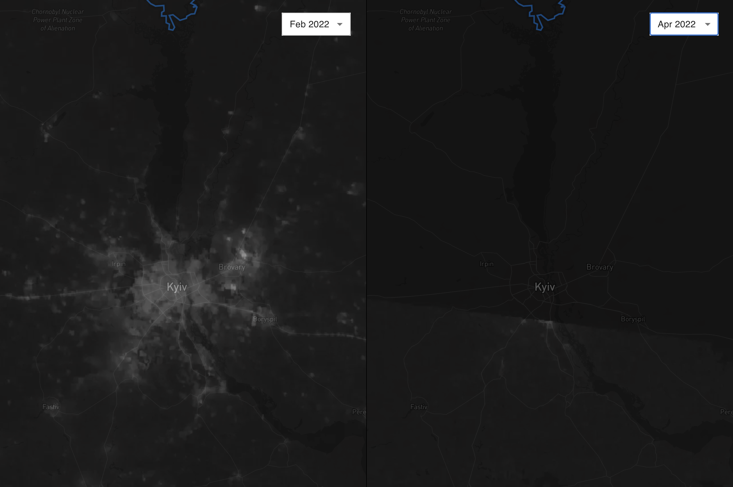
In light of the recent geopolitical events, I have developed a web-based GIS dashboard to visualize changes in nightlight output in Ukraine and its surroundings resulting from the ongoing Russian invasion.
Currently, this dashboard visualizes the night-sky of Ukraine before and after the Russian invasion. A nightly automated pipeline ensures the timely acquisition of new data and its subsequent publication.
Data source
The source data comes from the Colorado School of Mines, which provides tiff files on a monthly basis. These files present cloud-free composite images with a resolution of 15 arc-seconds, translating to an earthly resolution of approximately 450 meters by 450 meters at the equator.
It should be noted that the visualization tool does not incorporate data from the summer months. Due to the increased amount of light during these periods, sufficient data to construct monthly composites is lacking. For instance, an examination of Kyiv in April reveals the city largely shrouded in darkness. While there remains some residual light during these periods, it is not sufficiently captured by the source data.
Post-processing
The raw data used for this visualization required a number of post-processing steps to be suitably displayed. The code for these processes is written in Python and is openly available at this GitHub repository. The steps are as follows:
- Each element of the matrix M represents a roughly 450-meter by 450-meter area on Earth’s surface. To start, we clip these values such that they all lie within a specified range, defined by cliplower and clipupper . Each element Mij in the matrix is processed according to the following rule:
$$ \mathbf{M}_{ij} = \begin{cases} \text{{clip}}_{\text{{lower}}}, & \text{if } \mathbf{M}_{ij} < \text{{clip}}_{\text{{lower}}} \\ \text{{clip}}_{\text{{upper}}}, & \text{if } \mathbf{M}_{ij} > \text{{clip}}_{\text{{upper}}} \\ \mathbf{M}_{ij}, & \text{otherwise} \end{cases} $$
- We then apply a logarithmic transformation to every element of M. This transformation changes the data scale, helping to mitigate the effect of outliers. The numpy function
numpy.log10is used for this purpose; it applies a base-10 logarithm to each matrix element. To prevent any complications that might arise from taking the logarithm of zero, we add 1 to each element prior to applying the logarithm:
$$ \mathbf{M}_{ij} = \log_{10}(\mathbf{M}_{ij} + 1) $$
- After the logarithmic transformation, we rescale the data to span the range of an 8-bit integer, i.e., from 0 to 255. This is achieved using the
numpy.interpfunction, which performs linear interpolation. The base-10 logarithm of the upper clipping value, clipupper , and the lower clipping value, cliplower , are used as the bounds for rescaling:
$$ \mathbf{M}_{ij} = \frac{(\mathbf{M}_{ij} - \text{{clip}}_{\text{{lower}}}) \times 255}{\log_{10}(\text{{clip}}_{\text{{upper}}}) - \text{{clip}}_{\text{{lower}}})} $$
Conclusion
This open-source project is designed with adaptability in mind, allowing for the accommodation of alternative locations and post-processing techniques. If anyone feel like contributing to this project don’t hesitate to reach out or make a pull request.